Overview
During the summer camp, inspired by the concept of engineering robots in the RoboMaster Super League, each team was tasked with building a robot to complete the missions of collecting and exchanging minerals. My responsibility was designing the vision algorithm to meet the robot’s visual localization requirements.
I designed and implemented a real-time target pose estimation system (6 degrees of freedom) that runs on an embedded platform (Raspberry Pi 5). This system could calculate the 3D coordinates of the target (a yellow calibration board above the exchange slot) and transmit them to the downstream MCU via a serial port.
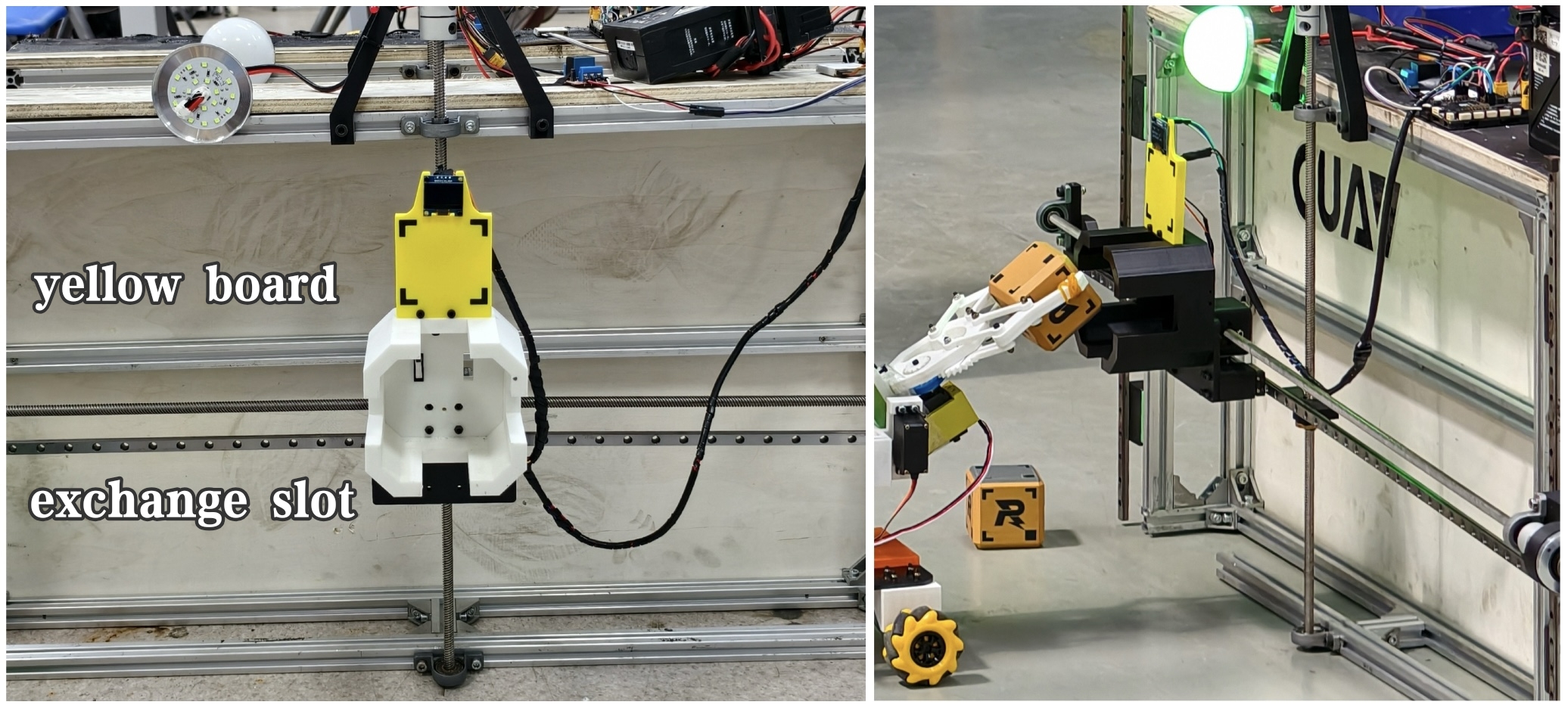
Initially, I adopted a purely traditional OpenCV-based approach, which combined mask filtering with the centroid method. However, during practical testing, I discovered that this algorithm was highly sensitive to environmental factors. Additionally, performing a full-frame search on high-resolution images incurred significant computational overhead.
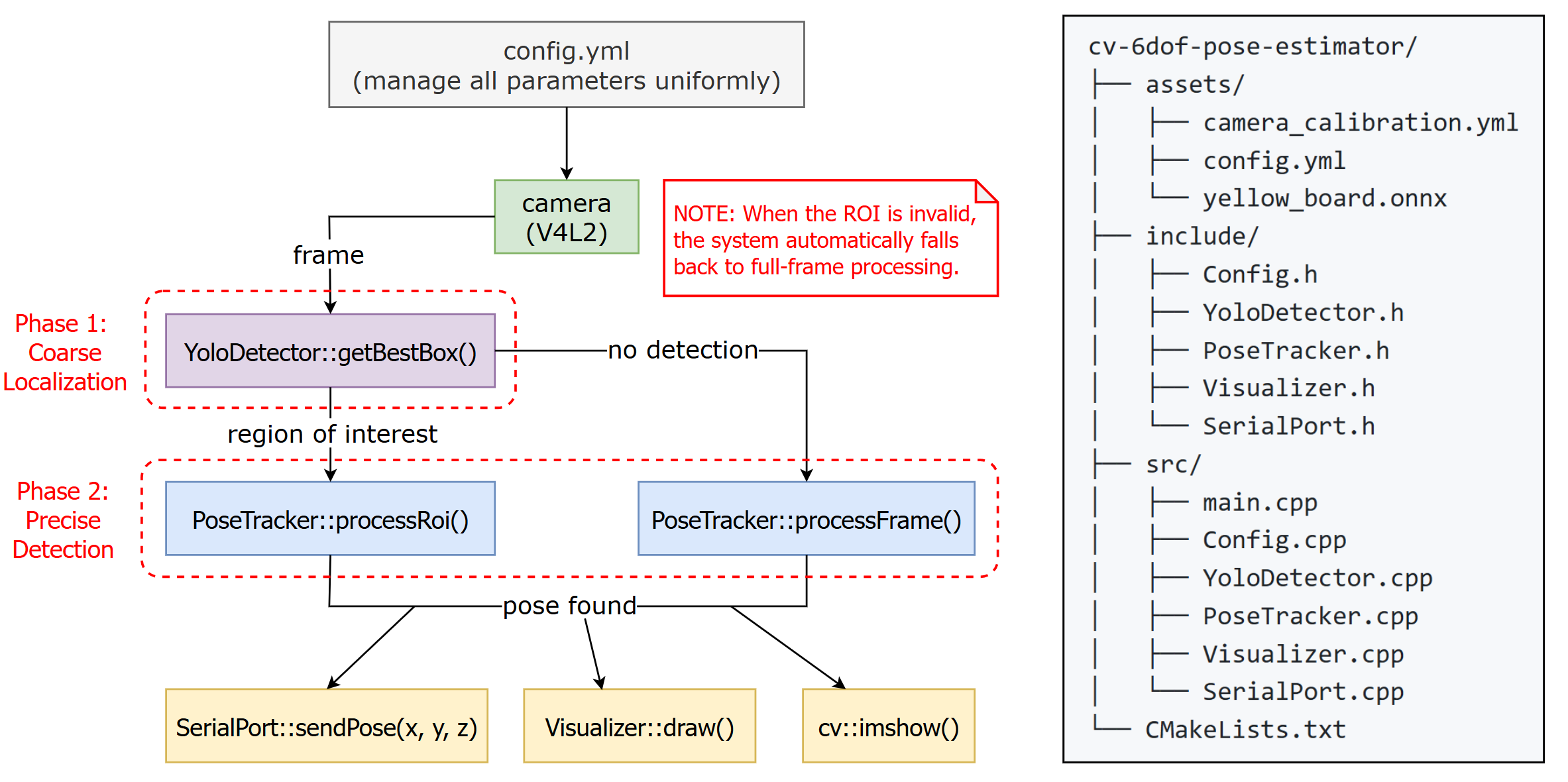
Therefore, I decided to incorporate deep learning into the solution. I trained a YOLO model to identify the calibration board region. This “Coarse Localization + Precise Detection” design offered three key advantages:
Improved Robustness: YOLO excels at handling complex backgrounds and partial occlusions. By first identifying the region of interest (ROI), it effectively filtered out background interference.
Accuracy Assurance: While deep learning models may not achieve sub-pixel precision in directly regressing corner coordinates, traditional geometric algorithms can. By retaining OpenCV’s sub-pixel corner detection, I ensured the geometric accuracy of the final pose estimation.
Optimized Computational Performance: Once the ROI was obtained using YOLO, OpenCV only needed to search for corner points within a very small image region, significantly reducing CPU computation.
Below is the overall Pipeline Diagram of the system:
Modules
Config
The Config module serves as the centralized parameter management layer for the entire system. Instead of hardcoding algorithm parameters, all tunable settings are externalized into a YAML configuration file ( assets/config.yml ). The system accepts three categories of parameters:
- Camera & Board: Device ID, capture resolution, path to camera calibration file, and the physical dimensions of the marker board.
TIP: If you switch cameras, simply update the config and calibration file without recompiling.
Marker Detection: HSV colour bounds for isolating the yellow board region, grayscale inversion threshold for locating dark corner markers, morphological kernel sizes for noise removal, and the minimum contour area to filter out spurious detections — These parameters are highly sensitive to lighting and background conditions in the deployment environment.
YOLO Detector: Model path, input resolution, confidence threshold, NMS threshold, and the extra padding around the detected ROI before feeding it to PoseTracker.
The Config class wraps OpenCV’s FileStorage API to parse YAML in a standard, cross-platform manner:
bool Config::loadConfig(const std::string &config_file_path)
{
    cv::FileStorage fs(config_file_path, cv::FileStorage::READ);
    // Parse camera settings
    fs["camera_id"] >> camera_id;
    fs["camera_width"] >> width;
    // ... parse detection parameters

    // Parse YOLO parameters with graceful degradation
    const cv::FileNode yolo_node = fs["yolo"];
    if (!yolo_node.empty()) {
        yolo_node["model_path"] >> yolo_params.model_path;
        // ... parse YOLO-specific settings
    } else {
        // Provide safe defaults if YOLO section is missing
        yolo_params.model_path = "";  // disables YOLO
    }
    return true;
}
The implementation follows a graceful degradation pattern: if the YOLO section is missing from the config file, the system logs a warning and assigns safe defaults, allowing the application to run without crashing.
YoloDetector
Model Training
1. Dataset Construction
Capture Environment: Images were recorded from the robot’s perspective, spanning multiple lighting conditions (indoor lighting, natural daylight, competition venue lighting), viewing angles (0° to 45° inclination), and distances (0.5 m to 3 m from the board).
Data Augmentation: To expand the dataset without manual recapture, I applied:
- Geometric Transforms: rotation (±15°) / scaling (0.8–1.2×) / horizontal flip
- Photometric Transforms: brightness adjustment (±20%) / contrast (±15%) / saturation (±10%)
- Dropout Augmentation: random erasing of image regions to simulate occlusion
This synthetic augmentation typically triples the effective dataset size.
Annotation Tool: I used labelImg, a popular open-source tool, to annotate the images. Each image’s annotation is stored in a
.txtfile with normalized bounding box coordinates:<class_id> <x_center> <y_center> <width> <height>. Since we have only one class,class_idis always 0.I partitioned the dataset as follows:
- Training set: 70% (~400 images after augmentation)
- Validation set: 20% (~100 images)
- Test set: 10% (~50 images, held out until final evaluation)
2. Finding the Best Model
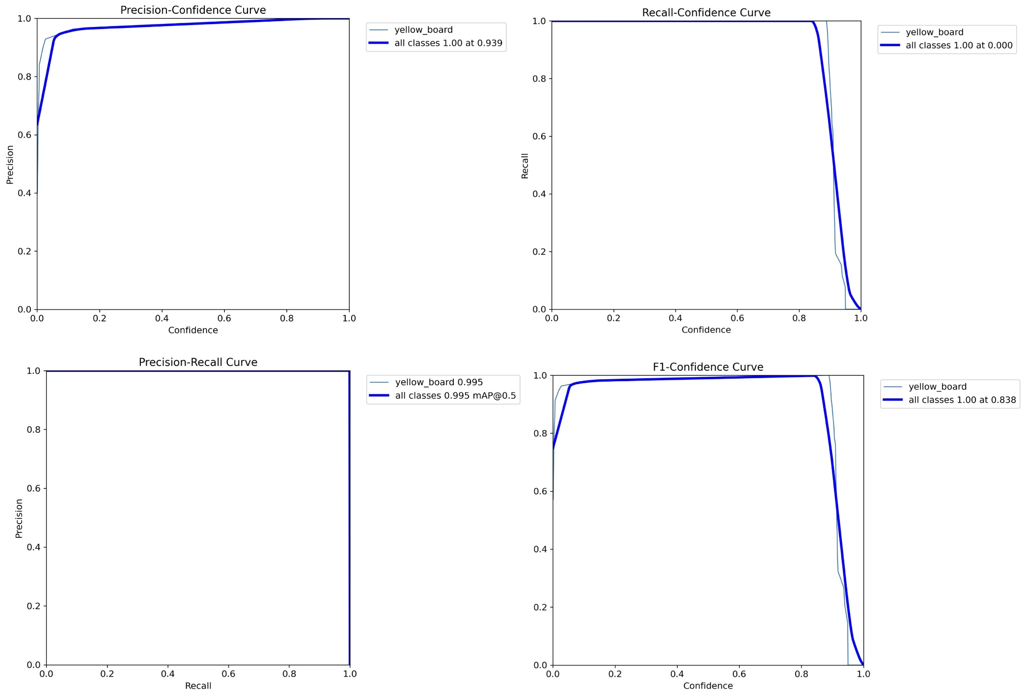
To identify the optimal model for this task, I experimented with six variants: YOLOv8n, YOLOv8s, YOLOv8m, YOLOv11n, YOLOv11s, and YOLOv11m. Each model was trained under identical conditions, and their performance was evaluated using the following metrics:
- P (Precision): Measures the proportion of true positives among all positive predictions.
- R (Recall): Measures the proportion of true positives among all actual positives.
- PR (Precision-Recall Curve): Visualizes the trade-off between precision and recall at different thresholds.
- F1 Score: The harmonic mean of precision and recall, providing a single metric for overall performance.
After analyzing the results, YOLOv11s achieved the best balance across all metrics:
I trained the model using the following configuration:
from ultralytics import YOLO

if __name__ == "__main__":
    model = YOLO(r"yolo11s.pt")
    model.train(
        data=r"yellow_board.yaml",  # Dataset configuration
        epochs=50,                   # Number of training epochs
        imgsz=640,                   # Input image size
        batch=-1,                    # Auto-adjust batch size
        cache="ram",                 # Cache dataset in RAM for faster training
        workers=1,                   # Number of data loader workers
        project="result",            # Output directory
        name="yolo11s",              # Experiment name
    )
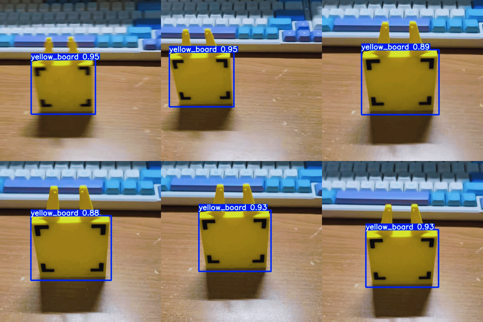
The training process was visualized in real-time, and the final results demonstrated significant improvements in both precision and recall:
3. Exporting to ONNX Format
YOLOv11 models are trained in PyTorch format (.pt), but the C++ inference runtime expects ONNX (Open Neural Network Exchange) format for cross-platform portability. Export is straightforward:
model = YOLO('best.pt')
model.export(format='onnx', imgsz=640, opset=12, simplify=True)
The exported ONNX model expects input shape [1, 3, 640, 640] (batch size 1, RGB channels, 640×640 pixels) and outputs [1, 4 + num_classes, num_anchors] — exactly what the YoloDetector’s postprocess() expects.
Inference Pipeline
The YoloDetector follows a standard three-step inference pattern:
Input Frame (1280×720, BGR)
        │
        ▼ preprocess()
        │  · Compute uniform scale: min(640/1280, 640/720) ≈ 0.889
        │  · Resize to 1138×640, centre on 640×640 grey canvas (114,114,114)
        │  · Compute offset: (51, 0) for letterbox padding
        │  · Normalize [0, 255] → [0, 1]
        │  · BGR → RGB via swapRB flag
        │  · blobFromImage: HWC to CHW, dtype float32
        │
        ▼ blob [1, 3, 640, 640] -- (1 batch, 3 channels, H×W)
        │
        ▼ net_.forward() -- (Runs YOLOv11s inference on GPU/CPU)
        │
        ▼ output [1, 4 + num_classes, num_anchors] -- (Raw tensor from ONNX model)
        │
        ▼ postprocess()
        │  ① Reshape [1, 4+nc, anchors] → [4+nc, anchors]
        │  ② Transpose → [anchors, 4+nc] -- (each row = one anchor)
        │  ③ For each anchor:
        │     · Find argmax class: max(row[4:4+nc])
        │     · Filter: if max_score < conf_thresh (0.50) → skip
        │     · Reverse letterbox: cx_frame = (cx_blob - offset.x) / scale
        │     · Convert centre → top-left: x = cx - w/2, y = cy - h/2
        │     · Clamp to frame bounds: [0, 1280]×[0, 720]
        │  ④ cv::dnn::NMSBoxes() removes overlaps (IoU > 0.40)
        │  ⑤ std::sort() by descending confidence
        │
        ▼ vector<Detection> -- (sorted by confidence)
        │  Each Detection: {box (x,y,w,h), confidence, classId}
        │
        ▼ getBestBox()
        │  Returns detections.front().box -- (highest confidence)
        │  or empty cv::Rect() if no detection survives
1. Preprocessing: Letterboxing for Precision
cv::Mat preprocess(const cv::Mat &frame, float &scale, cv::Point2f &offset) const
YOLO models trained with letterbox preprocessing must be inferred with the same preprocessing, otherwise coordinate mapping breaks down. The scale and offset computed are explicitly returned as output parameters and passed to postprocess() for coordinate transformation.
2. Postprocessing: Decoding the YOLO Tensor
(a) Reshape and Transpose
cv::Mat data = output.reshape(1, output.size[1]);
cv::transpose(data, data);
- Each row is one anchor prediction:
[1, 4 + nc, anchors] → [4 + nc, anchors] → [anchors, 4 + nc] - First 4 channels: box centre (cx, cy) and size (w, h) in the 640×640 blob coordinate system.
(b) Find the Argmax Class
For each anchor, identify the class with the highest confidence:
float max_score = 0.f;
int best_cls = 0;
for (int c = 0; c < num_classes; ++c) {
    if (row[4 + c] > max_score) {
        max_score = row[4 + c];
        best_cls = c;
    }
}
This allows the system to handle multi-class scenarios (in this project, we only care about the “yellow board” class).
(c) Coordinate Transformation
// Remove letterbox offset
cx_frame = (cx_blob - offset.x) / scale;
cy_frame = (cy_blob - offset.y) / scale;
bw_frame = bw_blob / scale;
bh_frame = bh_blob / scale;

// Convert from centre format to top-left format
x = cx_frame - bw_frame / 2;
y = cy_frame - bh_frame / 2;
This inverse transformation is the sine qua non of correct multi-scale detection — get it wrong by even a few pixels, and the downstream PoseTracker will search in the wrong ROI.
(d) Boundary Clamping
x = clamp(x, 0, frame.width - 1);
y = clamp(y, 0, frame.height - 1);
w = clamp(w, 1, frame.width - x);
h = clamp(h, 1, frame.height - y);
This prevents out-of-bounds array access when the model predicts boxes that partially lie outside the frame.
(e) Non-Maximum Suppression (NMS)
cv::dnn::NMSBoxes(boxes, confidences, conf_thresh_, nms_thresh_, indices);
conf_thresh_: filters out detections below a confidence cutoff (default 0.50)nms_thresh_: suppresses overlapping boxes with IoU > 40% (default 0.40)
(f) Sorting by Confidence
The results are sorted in descending confidence order, so the highest-confidence detection can be trivially extracted via getBestBox(), which simply returns detections.front().box.
3. Integration with PoseTracker
After YOLO detection, the best bounding box is passed to PoseTracker::processRoi(). The padding parameter in config.yml is crucial here — if the YOLO box is too tight, it may crop the corner markers at the edges. The default 20-pixel expansion provides a safety margin.
PoseTracker
Corner Detection
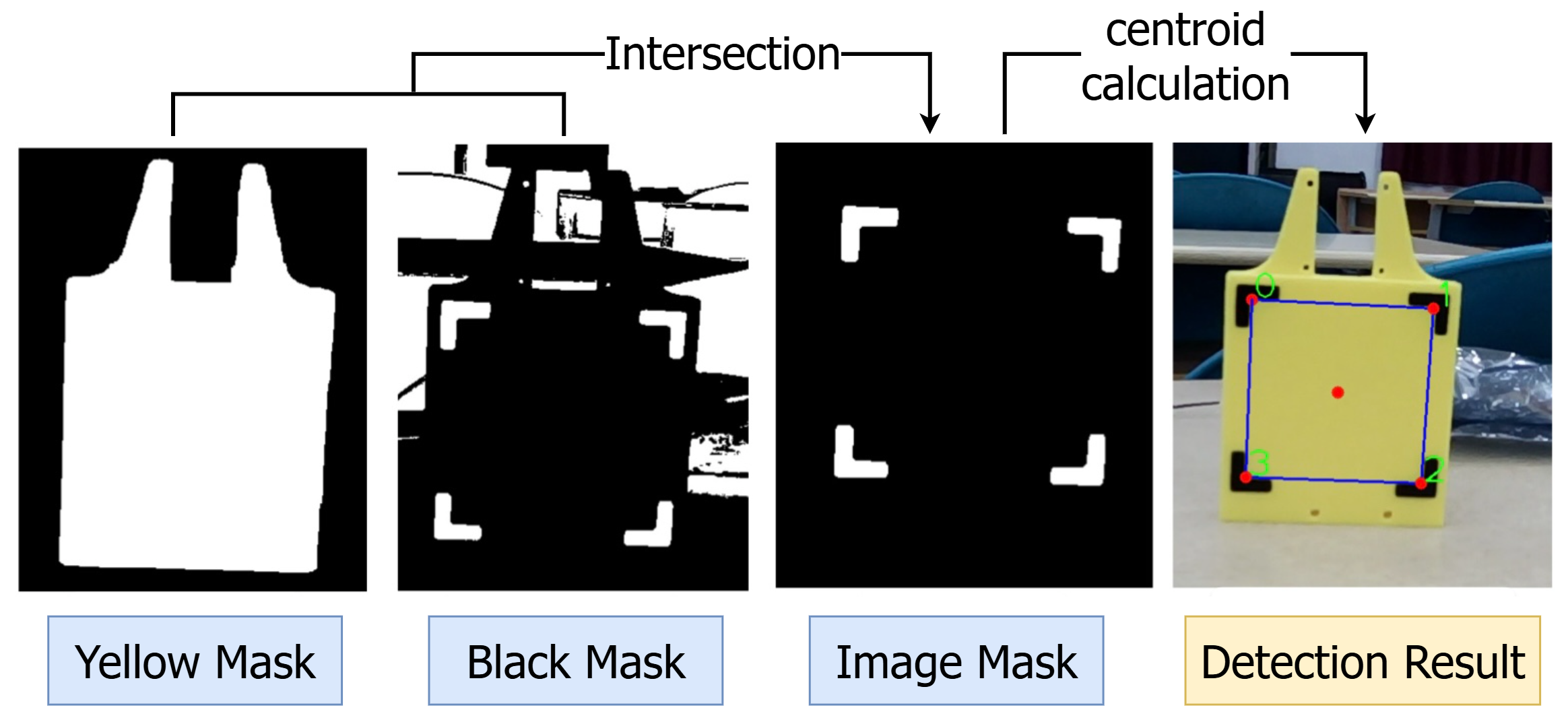
1. Yellow Region Extraction
cv::cvtColor(frame, imgHSV, cv::COLOR_BGR2HSV);
inRange(imgHSV, config.detector_params.hsv_yellow_lower,
        config.detector_params.hsv_yellow_upper, yellowMask);
cv::Mat kernel_large = getStructuringElement(cv::MORPH_RECT,
        cv::Size(config.detector_params.yellow_close_kernel_size, ...));
morphologyEx(yellowMask, yellowMask, cv::MORPH_CLOSE, kernel_large);
First, convert the frame to HSV colour space. HSV is far superior to RGB for colour-based segmentation because it separates colour information (H, S) from intensity (V), making it robust to lighting variations.
The inRange() call isolates pixels within the yellow HSV bounds.
However, due to shadows, compression artifacts, or uneven lighting, the yellow region may contain small dark holes. Morphological closing (a dilation followed by an erosion) bridges these gaps, filling small holes while preserving the outer boundary of the yellow region.
2. Dark Marker Extraction
cv::cvtColor(frame, imgGray, cv::COLOR_BGR2GRAY);
threshold(imgGray, blackMask, config.detector_params.grayscale_thresh_inv,
          255, cv::THRESH_BINARY_INV);
Separately, convert the frame to grayscale and apply inverse thresholding. The threshold value isolates pixels darker than this threshold. Inverse thresholding (THRESH_BINARY_INV) inverts the result, so dark regions become white (255).
3. Intersection and Denoising
bitwise_and(yellowMask, blackMask, imgMask);
cv::Mat kernel_small = getStructuringElement(cv::MORPH_RECT,
        cv::Size(config.detector_params.marker_open_kernel_size, ...));
morphologyEx(imgMask, imgMask, cv::MORPH_OPEN, kernel_small);
The intersection of these two masks (bitwise_and) yields the “black-on-yellow” markers.
Morphological opening (an erosion followed by a dilation) then removes small noise blobs that survived the prior filters. The kernel size is small to avoid eroding the actual marker corners.
4. Contour-Based Corner Localization
For each connected component (contour) in the binary mask:
- Area filtering: Discard contours with area <
min_marker_areato reject noise. - Centroid calculation: Compute the geometric centroid of the contour using moments.
- Representative corner point: For each contour, find the contour point closest to the centroid. This provides a sub-pixel estimate that’s more stable than simply taking the contour’s bounding-box corners.
Finally, accept the detection only if exactly four corners are found.
5. Corner Reordering for Consistency
The reorderCorners() method imposes a canonical ordering on the four detected corners:
- Top-left: Minimizes x + y (sum is smallest in upper-left)
- Top-right: Maximizes x − y (difference is largest when x » y)
- Bottom-right: Maximizes x + y (sum is largest in lower-right)
- Bottom-left: Minimizes x − y (difference is smallest when y » x)
This ordering ensures consistent correspondence between the detected 2D corners and the pre-computed 3D model.
Pose Estimation
Once four accurate 2D-3D correspondences are established, estimatePose() invokes OpenCV’s PnP solver:
void PoseTracker::estimatePose()
{
    cv::solvePnP(boardCorners3D, boardCorners2D, cameraMatrix, distCoefficients,
                 r_vec, t_vec);
}
Inputs
boardCorners3D: Four known 3D corner positions in board space (in metres, Z = 0).boardCorners2D: The four detected 2D corners in image space (in pixels).cameraMatrix: 3×3 intrinsic camera matrix from calibration.distCoefficients: Lens distortion coefficients from calibration.
Outputs:
r_vec: 3-element rotation vector (Rodrigues representation), encoding the 3×3 rotation matrix.t_vec: 3-element translation vector (in metres), representing the position of the board’s origin relative to the camera.
What is PnP ? Perspective-n-Point is a classical problem in computer vision: given n known 3D points and their projections onto the image plane, recover the camera’s pose (rotation and translation) relative to the 3D coordinate system.
ROI Processing
The processRoi() method extends the full-frame logic to handle YOLO’s bounding-box output:
bool PoseTracker::processRoi(const cv::Mat &frame, const cv::Rect &roi)
{
    // Validate ROI; fall back to full-frame processing if invalid.
    cv::Rect safe_roi = roi & cv::Rect(0, 0, frame.cols, frame.rows);
    if (safe_roi.empty())
        return processFrame(frame);

    // Run corner detection on the cropped sub-image.
    cv::Mat cropped = frame(safe_roi);
    findCorners(cropped);

    if (!boardCorners2D.empty())
    {
        // Map detected corners from ROI-local coords back to full-frame coords.
        for (auto &pt : boardCorners2D)
        {
            pt.x += static_cast<float>(safe_roi.x);
            pt.y += static_cast<float>(safe_roi.y);
        }
        estimatePose();
        isPoseFound = true;
    } else {
        isPoseFound = false;
    }
    return isPoseFound;
}
This design enables the two-stage pipeline: YOLO reduces the search space, PoseTracker performs precise corner detection within that reduced space, and the coordinate mapping ensures correctness.
Visualizer
Rendering Flow
draw()
  ├─→ drawStatus()          [Always: "Tracking" or "Searching..."]
  └─→ if (isTargetFound)
       ├─→ drawDetection()  [Quadrilateral + corner circles + centroid]
       └─→ drawPose()       [3D axes via projectPoints() + numerical text]
3D-to-2D Projection
The technical part of visualization involves converting 3D board-space coordinates to 2D image coordinates:
cv::projectPoints(axisPoints3D,     // 3D axis endpoints (0.02m along each axis)
                  r_vec,            // Rotation from PnP
                  t_vec,            // Translation from PnP
                  cameraMatrix,     // Camera intrinsics
                  distCoefficients, // Lens distortion
                  axisPoints2D);    // Output: 2D projected points
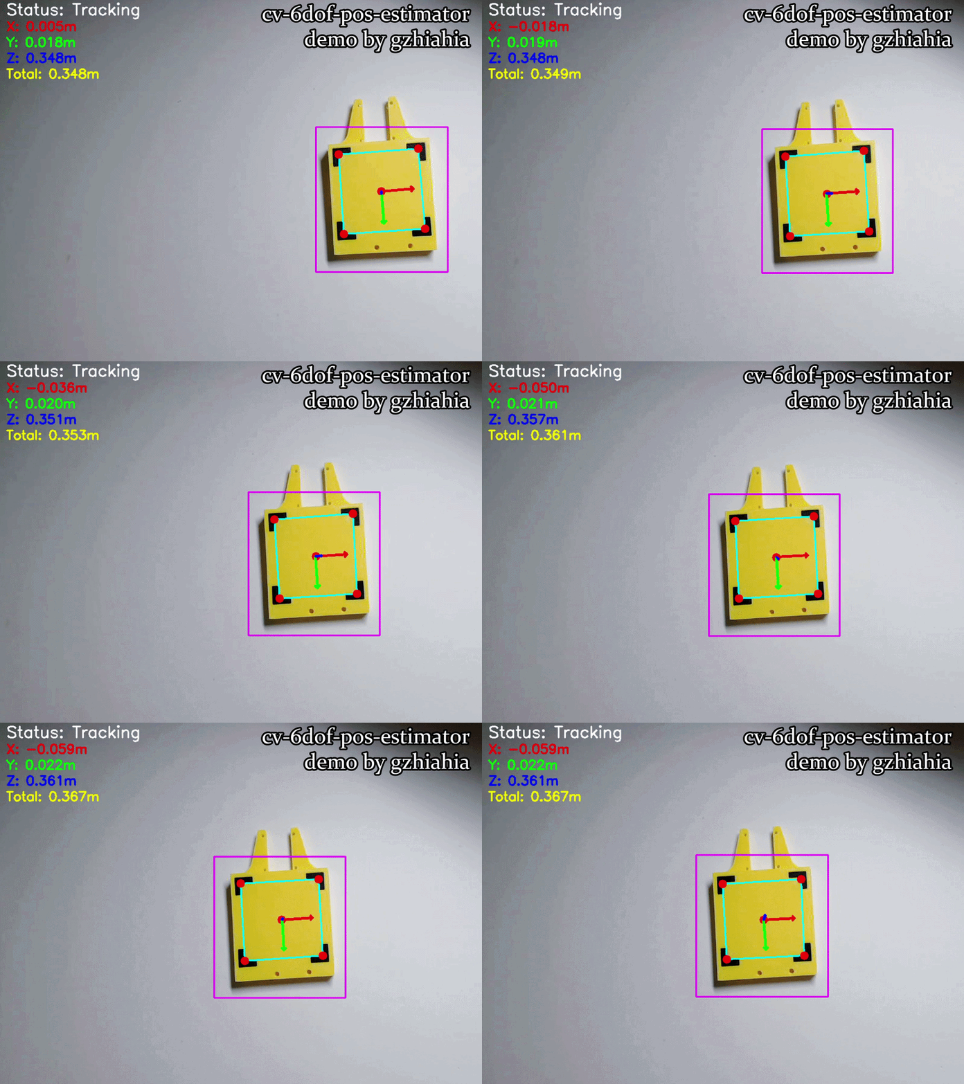
The Visualizer renders multiple layers of information, each serving a specific diagnostic or informational purpose:
| Element | Color | Type | Location | Purpose |
|---|---|---|---|---|
| Status Text | White | Text | Top-left (20, 30) | “Tracking” or “Searching…” feedback |
| X-axis Arrow | Red | Arrow (3px) | From origin | Left-right motion indicator |
| Y-axis Arrow | Green | Arrow (3px) | From origin | Up-down motion indicator |
| Z-axis Arrow | Blue | Arrow (3px) | From origin | Forward-backward indicator |
| Total Distance | Yellow | Text | Top-left (20, 150) | Euclidean distance to the board |
| YOLO Bounding Box | Purple | Rectangle (2px) | Around ROI | Coarse detection region (from main.cpp) |
| Corner Markers | Red | Circles (r=8px) | At each corner | Highlights precise corner localization |
| Corner Quadrilateral | Cyan | Lines (2px) | On board | Connects four corners & shows board orientation |
| Centroid Marker | Red | Circle (r=8px) | Board centre | Reference point for board position |
Raspberry Pi 5
SerialPort
The SerialPort module encapsulates serial communication logic, enabling the pose estimation results to be transmitted to a downstream embedded controller (e.g. robot’s motor control MCU).
Protocol Design
The pose transmission format is deliberately minimalist (3-DoF translation):
S,<x>,<y>,<z>,E\n
If full 6-DoF transmission becomes necessary, the protocol can be extended without refactoring:
- The PoseTracker module calculates the rotation vector (
r_vec) viacv::solvePnP() - The
getRotationVector()interface provides direct access to this data - Converting to Euler angles or quaternions is straightforward
// Optional 6-DoF extension:
S,<x>,<y>,<z>,<roll>,<pitch>,<yaw>,E\n
// or with quaternions:
S,<x>,<y>,<z>,<qw>,<qx>,<qy>,<qz>,E\n
The default serial port and baud rate are hardcoded (To be optimized: set in Config module) in main.cpp:
SerialPort communicator("/dev/ttyAMA4", 115200);
However, this is easily customized for different hardware:
// USB-to-serial adapter (common on PC)
SerialPort communicator("/dev/ttyUSB0", 115200);

// Lower baud rate for long cables or noisy environments
SerialPort communicator("/dev/ttyAMA4", 9600);

// Windows COM port
SerialPort communicator("COM3", 115200);
Implementation
The SerialPort class wraps Boost.Asio’s serial port functionality:
SerialPort::SerialPort(const std::string &port_name, unsigned int baud_rate)
    : m_io_service(), m_port(m_io_service)
{
    try {
        m_port.open(port_name);
        // Configure 8N1: 8 data bits, no parity, 1 stop bit
        m_port.set_option(boost::asio::serial_port_base::baud_rate(baud_rate));
        m_port.set_option(boost::asio::serial_port_base::character_size(8));
        m_port.set_option(boost::asio::serial_port_base::parity(boost::asio::serial_port_base::parity::none));
        m_port.set_option(boost::asio::serial_port_base::stop_bits(boost::asio::serial_port_base::stop_bits::one));
        m_port.set_option(boost::asio::serial_port_base::flow_control(boost::asio::serial_port_base::flow_control::none));
        std::cout << "Serial port opened at " << baud_rate << " baud." << std::endl;
    } catch (const boost::system::system_error &e) {
        std::cerr << "Error opening serial port: " << e.what() << std::endl;
    }
}
Transmission (To be optimized)
The sendPose() method formats and transmits a pose packet:
bool SerialPort::sendPose(double x, double y, double z)
{
    if (!m_port.is_open())
        return false;

    std::stringstream ss;
    ss << "S," << x << "," << y << "," << z << ",E\n";
    std::string data = ss.str();

    try {
        boost::asio::write(m_port, boost::asio::buffer(data));
        return true;
    } catch (const boost::system::system_error &e) {
        std::cerr << "Error sending data: " << e.what() << std::endl;
        return false;
    }
}
- Synchronous write:
boost::asio::write()blocks until all bytes are sent. - String formatting:
std::stringstreamprovides automatic float-to-ASCII conversion with default precision. - Buffer management:
boost::asio::buffer()wraps the string’s internal buffer; no additional memory allocation occurs.
Future Extensions
- Asynchronous writes ! Use
async_write()to avoid blocking the main vision loop - Bidirectional protocol: MCU sends pose confirmation; Pi retransmits on timeout
- Confidence fields: Add corner detection score → MCU adjusts control gains
Deployment
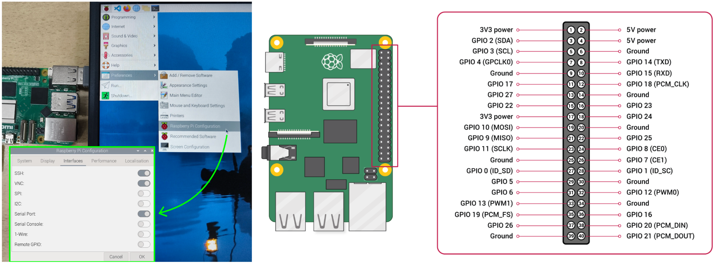
1. Serial Port Settings
dtoverlay -a | grep uart
dtoverlay -h uart4

sudo vim /boot/firmware/config.txt
# Add "dtoverlay=uart4" at the end
sudo reboot

ls /dev/ttyAMA*
# "/dev/ttyAMA4" should appear
2. Hardware Connection
GPIO14 = TXD0 -> ttyAMA0
GPIO0  = TXD2 -> ttyAMA1
GPIO4  = TXD3 -> ttyAMA2
GPIO8  = TXD4 -> ttyAMA3
GPIO12 = TXD5 -> ttyAMA4 [√]

GPIO15 = RXD0 -> ttyAMA0
GPIO1  = RXD2 -> ttyAMA1
GPIO5  = RXD3 -> ttyAMA2
GPIO9  = RXD4 -> ttyAMA3
GPIO13 = RXD5 -> ttyAMA4 [√]
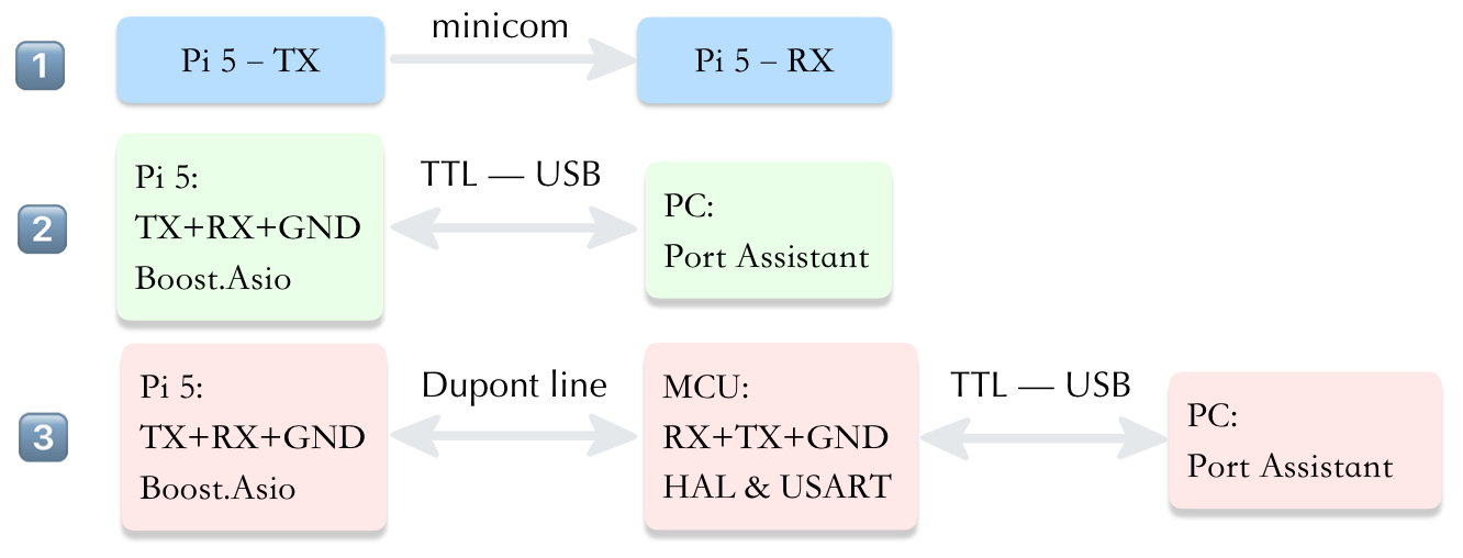
3. Debugging
sudo apt-get install minicom
sudo minicom -D /dev/ttyAMA4 -b 115200